Deep Learning - Convolutional Neural Network

Bhaskar S

02/22/2025

Introduction

In the article Introduction to Deep Learning - Part 2 of the Deep Learning series, we provided an intuition on the inner workings of a Feed Forward neural network.

Can one use a Feed Forward neural network for classifying images/pictures - Absolutely one can !

However, it will be very resource (compute and memory) intensive - Why ?

Let us consider we have a collection of 32 pixel by 32 pixel images of 5 fruits, say, apple, banana, mango, orange, and pear. The number of input features to the Feed Forward neural network would be $32 \times 32 = 1024$.

If the Feed Forward neural network has two hidden layers of $512$ neurons each and an output layer of $5$ neurons (one for each fruit), we will end up with a total of $1024 \times 512 \times 512 \times 5 = 1342177280$ OR approximately $1.3$ Billion parameters.

This is where the Convolutional Neural Network (or CNN for short) comes into play !!!

Convolutional Neural Network

Before we get started, we need to understand some fundamental concepts related to the CNN model.

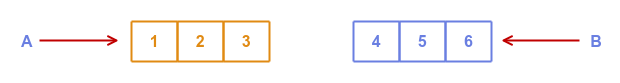
Let $A$ and $B$ be two vectors as shown in the illustration below:

Cross Correlation is a mathematical measure of similarity between the two vectors.

In mathematical terms:

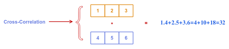
$a_n * b_n = \sum_{i=0}^{n-1} a[i].b[i]$

The following illustration depicts the cross correlation between vectors $A$ and $B$:

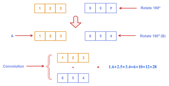
Convolution is a mathematical operation that combines the two vectors to find overlapping patterns between them.

In mathematical terms:

$a_n * b_n = \sum_{i=0}^{n-1} a[i].rotate_{180}(b[i])$

The following illustration depicts the convolution between vectors $A$ and $B$:

A full convolution is a mathematical operation that combines the two vectors by sliding one vector over the other to find overlapping patterns between them.

The following illustration depicts the full convolution between vectors $A$ and $B$:

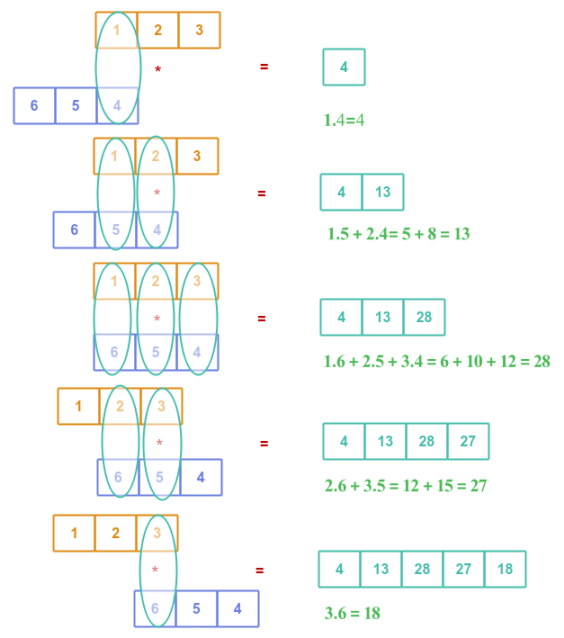
Given vector $A$ of size $n$ and vector $B$ of size $m$ where $m \le n$, then a full convolution will generate a third vector $C$ of size $n + m - 1$.

The concept of convolution is not just limited to vectors. It can also be applied to matrices (a 2-dimensional structure).

The $A$ is a matrix of dimensions $n \times n$ and $B$ a smaller matrix of dimensions $m x m$, then the output matrix $C$ from the convolution of $A$ and $B$ will be of dimensions $(n - m + 1) \times (n - m + 1)$. The output matrix $C$ is often referred to as the Feature Map.

The smaller matrix $B$ that slides over the matrix $A$ is often referred to as a Kernel or a Filter.

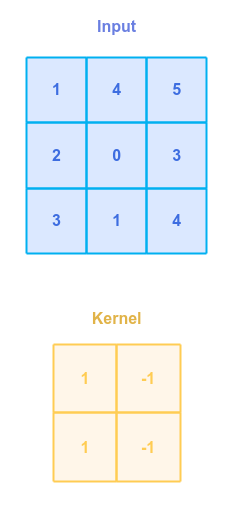
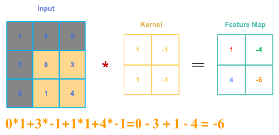
The following illustration shows the input matrix $A$ and the kernel matrix $B$ that will be used to compute the output feature map matrix:

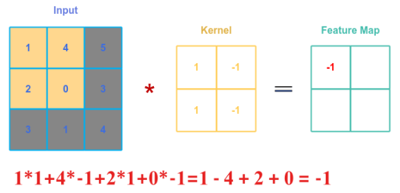
The following illustration shows applying the convolution between the kernel matrix $B$ and the top left part of matrix $A$:

Sliding the kernel matrix $B$ by certain number of offsets is referred to as the Stride. For our example, we will use a stride of $1$, meaning we will slide the kernel matrix $B$ by one offset at a time.

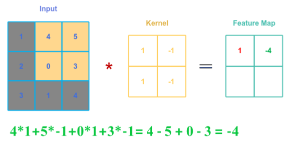
The following illustration shows applying the convolution between the kernel matrix $B$ and the top right part of matrix $A$ after sliding one offset to the right:

If the $A$ is a matrix of dimensions $n \times n$, the kernel matrix $B$ is of dimensions $m \times m$, and stride $s$ denotes the number of offsets by which the kernel slides, then the output matrix $C$ from the convolution of $A$ and $B$ with a stride $s$ will be of dimensions $\Large{\frac{(n-m)}{s}}$$+1 \times \Large{\frac{(n-m)}{s}}$$+1$.

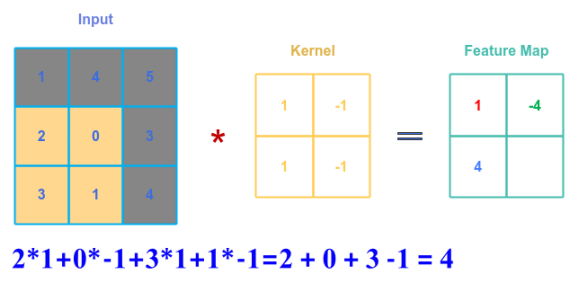
The following illustration shows applying the convolution between the kernel matrix $B$ and the lower left part of matrix $A$ after sliding one offset down:

Finally, the following illustration shows applying the convolution between the kernel matrix $B$ and the lower right part of matrix $A$ after sliding one offset to the right:

One observation from the convolution between matrix $A$ and the kernel matrix $B$ - the patterns in the sections of the matrix $A$ away from the edges is covered more than the one along the edges.

The following illustration depicts this situation:

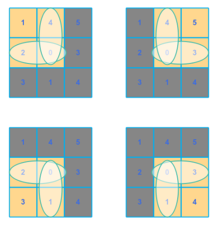
If we consider the matrix $A$ as a representation of an image, there may be some patterns along the edges that may not be well captured by the convolution operation.

To solve for this, one could insert additional cell(s) along the edges (could be one or more) . This technique is referred to as Padding. The following illustration depicts padding of one:

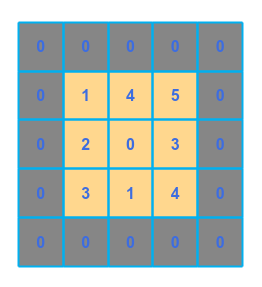
Typically, the padding is done with zeros.

With the padding of one to matrix $A$ and a stride of one, the following illustration depicts the convolution operations for the first few steps (follow the red circled numbers):

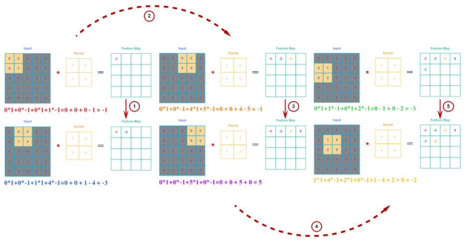
If the $A$ is a matrix of dimensions $n \times n$, the kernel matrix $B$ is of dimensions $m \times m$, with padding of $p$, and a stride of $s$, then the output matrix $C$ from the convolution of $A$ and $B$ will be of dimensions $\Large{\lfloor{ \frac{(n+2.p-m)}{s}}}$$+1 \rfloor \times \Large{\lfloor{\frac{(n+2.p-m)}{s}}}$$+1 \rfloor$.

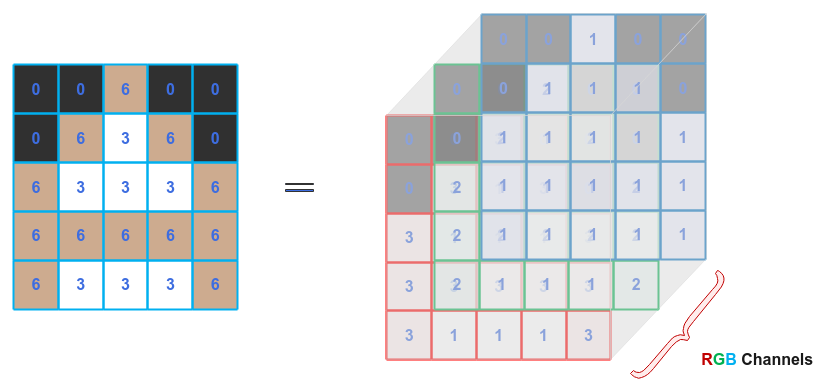
As indicated earlier, an image is made up of a grid of pixels and each of the pixels are a combination of three base colors often referred to as the RGB (Red, Green, Blue) Channels.

Often times the channels are referred to as the Depth, which is often confusing. In this article, we will instead use the term Channels.

The following illustration shows how an image (on the left) can be represented as a tensor (multi dimensional) of $3$ RGB channels:

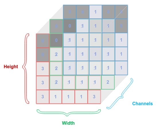
Now that we understand that an imgae can be represented as as a tensor, the following illustration highlights the various attributes of the image tensor:

The convolution operation can be performed on an input tensor (with 3 channels) using a kernel tensor (with 3 channels) such that the output is the sum of $3$ convolution operations, one from each of the channels from the input tensor with the corresponding channels from the kernel tensor. The following illustration depicts this scenario:

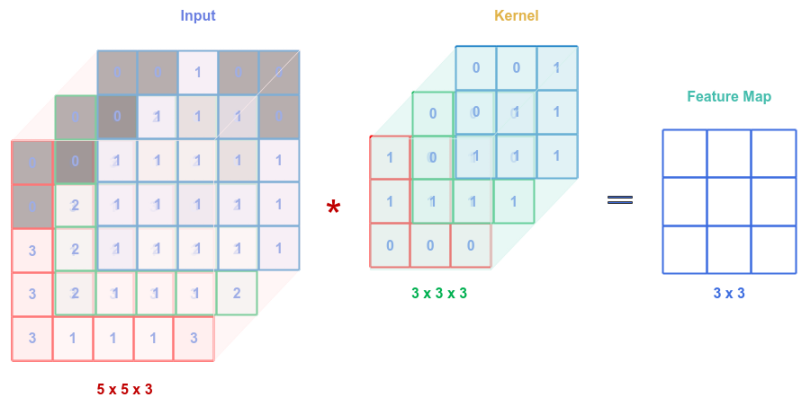
Note that the number channels in the input tensor and the kernel tensor MUST match.

A kernel (or filter) tensor (with 3 channels) is used for detecting patterns in the input tensor (with 3 channels). Nothing is preventing one from using multiple kernels (or filters) to detect different patterns from the input tensor. The following illustration depicts this scenario:

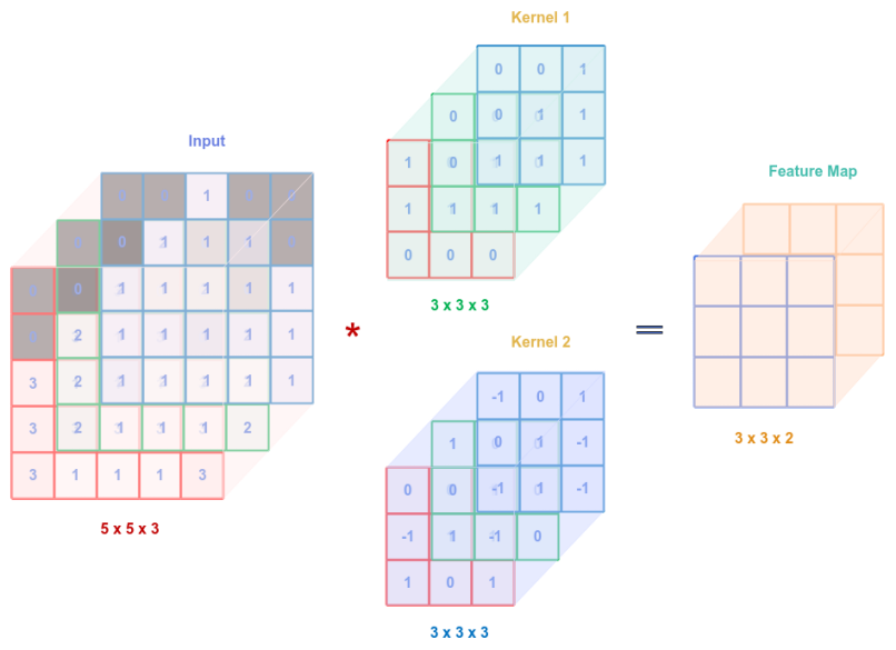
If the number of kernel tensors used is $k$, then the output feature map tensor will have a depth of $k$. In the above case, we used $2$ kernels, hence the output feature map tensor has a depth of $2$.

A layer in the neural network that consists of a convolution operation between an input tensor and a set of kernel tensors is often referred to as a Convolutional Layer.

If added a bias to each of the output from a kernel (or filter) tensor and run it through an activation function $\alpha$, we will get a transformed feature map output. The following illustration depicts this case:

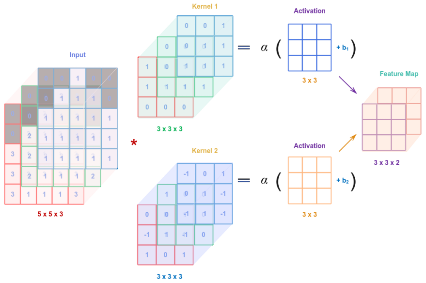
Comparing the above illustration to the Feed Forward neural network, we observe some similarities, where the input image represented as a tensor (of pixel values) is combined with the weights from the kernel tensor(s), then combined with bias parameters, and finally processed by an activation function $\alpha$ to form an intermediate tensor that could be passed to the next layer.

Although it may appear as though a convolution layer appears to reduce the dimensions of the input tensor, however, it is not the primary intent of a convolution layer, but more for feature extraction using a set of kernels (or filters).

A Pooling operation uses a kernel (or filter) to reduce a set of features to a single feature. There are two types of pooling operation - Max Pooling and Average Pooling. The commonly used pooling kernel is the max pooling as it works well in the real world.

The following illustration depicts both the max pooling and average pooling cases using a stride of $2$:

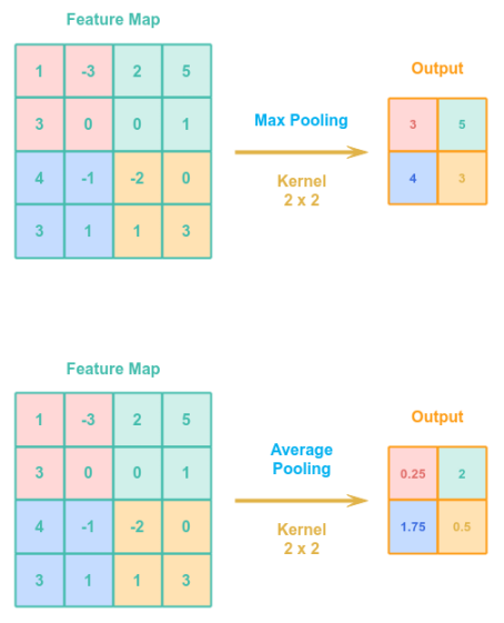
Given the pooling kernel is 2 x 2, in the case of max pooling, the kernel picks the maximum value from the shaded region of the input. For the average pooling, the kernel avergaes the values from the shaded region.

At this point, we have covered all the core concepts for building a convolutional neural network.

The following illustration depicts how one can compose a convolutional neural network that ultimately feeds into a dense feed forword network:

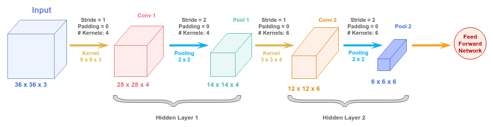
Note that the convolutional operation and the pooling operation together form a hidden layer.

Hands-on CNN Using PyTorch

We will demonstrate how one could leverage the CNN model for classifying the handwritten digits from the MNIST dataset, which consists of about handwritten digit images of size 28 x 28 in grayscale.

To import the necessary Python module(s), execute the following code snippet:

import torch

import matplotlib.pyplot as plt

import torch.nn.functional as F
import torchvision.datasets as datasets
import torchvision.transforms as transforms

from torch import optim
from torch import nn
from torch.utils.data import DataLoader

In order to ensure reproducibility, we need to set the seed to a constant value by executing the following code snippet:

seed_value = 3

torch.manual_seed(seed_value)

To download the MNIST data to the directory ./data, execute the following code snippet:

data_dir = './data'

train_dataset = datasets.MNIST(root=data_dir, download=True, train=True, transform=transforms.ToTensor())
test_dataset = datasets.MNIST(root=data_dir, download=True, train=False, transform=transforms.ToTensor())

The above code snippet will ONLY download the MNIST dataset once.

The MNIST dataset has $10$ digits from $0$ to $9$ and hence we need $10$ classes. Our CNN model will use $2$ convolutional layers, with the first layer with $8$ kernels and the second layer with $16$ kernels. Each kernel will be of size $3 \times 3$, with a padding of $1$ and a stride of $1$. In addition, our CNN model will use a common Max Poolinng kernel of size $2 \times 2$ and a stride of $2$ for the two layers. To initialize the variables for our CNN model hyperparameters, execute the following code snippet:

# No of digits to classify
num_classes = 10

# Common Max Pooling for all Layers
pool_k = 2 # Max Pooling Kernel size
pool_s = 2 # Max Pooling Stride

# Layer 1 Convolution
l1_in_ch = 1 # Layer 1 Convolution No of channels
l1_c_k = 3 # Layer 1 Convolution Kernel size
l1_c_s = 1 # Layer 1 Convolution Stride
l1_c_p = 1 # Layer 1 Convolution Padding
l1_c_num_k = 8 # Layer 1 Convolution No of Kernels

# Layer 2 Convolution
l2_in_ch = l1_c_num_k # Layer 2 Convolution No of channels
l2_c_k = l1_c_k # Layer 2 Convolution Kernel size
l2_c_s = l1_c_s # Layer 2 Convolution Stride
l2_c_p = l1_c_p # Layer 2 Convolution Padding
l2_c_num_k = 16 # Layer 2 Convolution No of Kernels

# Fully Connected Feed Forward
ff_in_ch = l2_c_num_k
ff_sz = 7 * 7

To define our CNN model, execute the following code snippet:

class CNN(nn.Module):
  def __init__(self):
    super(CNN, self).__init__()

    # Common Max Pooling used in Layer 1 and Layer 2:
    #   Kernel size: 2 x 2
    #   Stride: 2
    self.pool = nn.MaxPool2d(kernel_size=pool_k, stride=pool_s)

    # Convolutional Layer - 1:
    #   No. of channels: 1
    #   Kernel size: 3 x 3
    #   Stride: 1
    #   Padding: 1
    #   No. of Kernels: 8
    #   Input size (h x w x c): 28 x 28 x 1
    #   Output size (after conv): n + 2.p - k + 1 = 28 - 2 - 3 + 1 = 28
    #   Output size (after pool): 28 / 2 = 14
    self.conv1 = nn.Conv2d(in_channels=l1_in_ch, out_channels=l1_c_num_k, kernel_size=l1_c_k, stride=l1_c_s, padding=l1_c_p)

    # Convolutional Layer - 2:
    #   No. of channels: 8
    #   Kernel size: 3 x 3
    #   Stride: 1
    #   Padding: 1
    #   No. of Kernels: 16
    #   Input size (h x w x c): 14 x 14 x 8
    #   Output size (after conv): n + 2.p - k + 1 = 14 - 2 - 3 + 1 = 14
    #   Output size (after pool): 14 / 2 = 7
    self.conv2 = nn.Conv2d(in_channels=l2_in_ch, out_channels=l2_c_num_k, kernel_size=l2_c_k, stride=l2_c_s, padding=l2_c_p)

    # Fully connected layer:
    #   Input size (h x w x c): 7 x 7 x 16
    #   Output size (after conv): n + 2.p - k + 1 = 14 - 2 - 3 + 1 = 14
    #   Output size (after pool): 14 / 2 = 7
    self.fc1 = nn.Linear(ff_sz * ff_in_ch, num_classes)

  def forward(self, x):
    # Layer 1
    # Conv followed by ReLU activation
    x = F.relu(self.conv1(x))
    # Max pooling
    x = self.pool(x)

    # Layer 2
    # Conv followed by ReLU activation
    x = F.relu(self.conv2(x))
    # Max pooling
    x = self.pool(x)

    # Flatten output from Layer 2 and feed into Fully connected layer
    x = x.reshape(x.shape[0], -1)
    x = self.fc1(x)

    return x

To initialize variables for the device to train on, the batch size of training samples, the learning rate, and the maximum number of epochs, execute the following code snippet:

device = 'cpu'
batch_sz = 64
learning_rate = 0.001
num_epochs = 10

To create an instance of the training and the test datasets and access the samples in batches via the dataloder, execute the following code snippet:

train_loader = DataLoader(dataset=train_dataset, batch_size=batch_sz, shuffle=True)
test_loader = DataLoader(dataset=test_dataset, batch_size=batch_sz, shuffle=True)

To create an instance of the CNN model, execute the following code snippet:

cnn_model = CNN().to(device)

To create an instance of the cross entropy loss, execute the following code snippet:

criterion = nn.CrossEntropyLoss()

To create an instance of the gradient descent optimizer, execute the following code snippet:

optimizer = optim.Adam(cnn_model.parameters(), lr=learning_rate)

To implement the iterative training loop to predict the class, compute the loss, and adjust the model parameters through backward pass, execute the following code snippet:

for epoch in range(num_epochs):
  print(f'Epoch -> {epoch}')
  for batch_index, (y_train, y_actual) in enumerate(train_loader):
    y_train = y_train.to(device)
    y_actual = y_actual.to(device)
    y_predict = cnn_model(y_train)
    loss = criterion(y_predict, y_actual)
    if batch_index % 450 == 0:
      print(f'\tCNN Model -> Batch: {batch_index}, Loss: {loss}')
    optimizer.zero_grad()
    loss.backward()
    optimizer.step()

The following would be a typical output:

Output.1

Epoch -> 0
  CNN Model -> Batch: 0, Loss: 2.3086910247802734
  CNN Model -> Batch: 450, Loss: 0.11928762495517731
  CNN Model -> Batch: 900, Loss: 0.16974475979804993
Epoch -> 1
  CNN Model -> Batch: 0, Loss: 0.05041820928454399
  CNN Model -> Batch: 450, Loss: 0.13513758778572083
  CNN Model -> Batch: 900, Loss: 0.07222650945186615
Epoch -> 2
  CNN Model -> Batch: 0, Loss: 0.11242908239364624
  CNN Model -> Batch: 450, Loss: 0.024590598419308662
  CNN Model -> Batch: 900, Loss: 0.07324884086847305
Epoch -> 3
  CNN Model -> Batch: 0, Loss: 0.03461407124996185
  CNN Model -> Batch: 450, Loss: 0.06733991950750351
  CNN Model -> Batch: 900, Loss: 0.051184553653001785
Epoch -> 4
  CNN Model -> Batch: 0, Loss: 0.11813825368881226
  CNN Model -> Batch: 450, Loss: 0.03529193252325058
  CNN Model -> Batch: 900, Loss: 0.11979389935731888
Epoch -> 5
  CNN Model -> Batch: 0, Loss: 0.011674241162836552
  CNN Model -> Batch: 450, Loss: 0.01464864332228899
  CNN Model -> Batch: 900, Loss: 0.07621130347251892
Epoch -> 6
  CNN Model -> Batch: 0, Loss: 0.014700329862535
  CNN Model -> Batch: 450, Loss: 0.004133279900997877
  CNN Model -> Batch: 900, Loss: 0.01158683467656374
Epoch -> 7
  CNN Model -> Batch: 0, Loss: 0.008119644597172737
  CNN Model -> Batch: 450, Loss: 0.004468552302569151
  CNN Model -> Batch: 900, Loss: 0.052064426243305206
Epoch -> 8
  CNN Model -> Batch: 0, Loss: 0.023992931470274925
  CNN Model -> Batch: 450, Loss: 0.006232535466551781
  CNN Model -> Batch: 900, Loss: 0.04387667030096054
Epoch -> 9
  CNN Model -> Batch: 0, Loss: 0.06665094941854477
  CNN Model -> Batch: 450, Loss: 0.014449195936322212
  CNN Model -> Batch: 900, Loss: 0.019443850964307785

To evaluate the trained CNN model using the test MNIST dataset samples, execute the following code snippet:

n_correct = 0
n_total = 0

cnn_model.eval()
with torch.no_grad():
  for y_test, y_actual in test_loader:
    y_test = y_test.to(device)
    y_actual = y_actual.to(device)
    y_predict = cnn_model(y_test)
    _, y_predict = y_predict.max(1)
    n_correct += (y_predict == y_actual).sum()
    n_total += y_predict.size(0)
  accuracy = float(n_correct) / float(n_total) * 100
  print(f'CNN Model -> Accuracy: {accuracy}')

The following would be a typical output:

Output.2

CNN Model -> Accuracy: 98.72999999999999

As can be inferred from the Output.2 above, the accuracy of the model is close to $99\%$ !!!

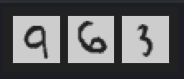
To display the 1st, 5th, and 9th digits from the test MNIST dataset samples, execute the following code snippet:

test_samples = enumerate(test_loader)
_, (samples, targets) = next(test_samples)

fig = plt.figure(figsize=(2, 6))
sp1 = fig.add_subplot(1, 3, 1)
sp1.set_xticks([])
sp1.set_yticks([])
sp1.imshow(samples[1][0], cmap='gray', interpolation='auto')
sp2 = fig.add_subplot(1, 3, 2)
sp2.set_xticks([])
sp2.set_yticks([])
sp2.imshow(samples[5][0], cmap='gray', interpolation='auto')
sp3 = fig.add_subplot(1, 3, 3)
sp3.set_xticks([])
sp3.set_yticks([])
sp3.imshow(samples[9][0], cmap='gray', interpolation='auto')
plt.show()

The following illustration shows the visual representation of the three selected digits:

To display what the trained CNN model predicted for the three selected digits, execute the following code snippet:

cnn_model.eval()
with torch.no_grad():
  y_predict = cnn_model(samples)
  _, y_predict = y_predict.max(1)
print(f'Predicted 1st, 5th, and 9th digit(s): {y_predict[1]}, {y_predict[5]}, {y_predict[9]}')

The following would be a typical output:

Output.3

Predicted 1st, 5th, and 9th digit(s): 9, 6, 3

BINGO - the trained CNN model seems to have classified the digits correctly !!!

References

PyTorch Documentation

Introduction to Deep Learning - Part 2