Deep Learning - The Vanishing Gradient

The Vanishing Gradient

In using a Neural Network for a complex use-case, one may simply assume that adding more number of hidden layers would solve the problem. But, there is an interesting challenge with this naive approach - the problem of the Vanishing Gradient.

In Part 1 of the deep learning series, we introduced the concept of the activation function and in particular the Sigmoid function.

A Sigmoid function is a non-linear activation function that squishes its output value to be in the range $[0, 1]$, for any given input value.

In mathematical terms:

$\sigma(x) = \Large{\frac{1}{1 + e^{-x}}}$

The following illustration shows the graph of a sigmoid activation function:

In Part 3 of the deep learning series, we found the derivative of a Sigmoid function to be:

$\Large{\frac{d\sigma}{dx}}$ $= \Large{\frac{d}{dx}}$ $\Large{(\frac{1}{1 + e^{-x}})}$ $=\Large{ \frac{d}{dx}}$ $(1 + e^{-x})^{-1}$ $= \sigma(x).(1 - \sigma(x))$

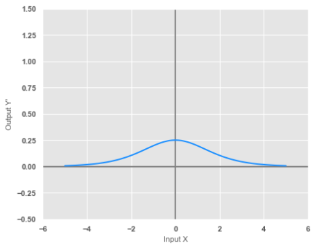
The following illustration shows the graph of the derivative of a sigmoid activation function:

Notice from the illustration in Figure.2 above, that the MAXIMUM value of the derivative of a sigmoid activation function is $0.25$.

To keep things simple, let us refer to the following illustration of the neural network with an input layer with two inputs, two hidden layers each consisting of two neurons, and an output layer with two outputs:

In Part 3 of the deep learning series, we went into the gory details of computing the gradients of the biases and weights with respect to the loss in order to optimize the model.

Let us consider the gradient of the weight $W_{1,1}^1$ with respect to the loss $L$.

In order to adjust the weight partameter $W_{1,1}^1$ during backpropagation, we need to compute the gradient for $\Large{\frac{\partial{L}}{\partial{W_{1,1}^1}}}$.

Once we have the gradient for $\Large{\frac{\partial{L}}{\partial{W_{1,1}^1}}}$, we can adjust the weight $W_{1,1}^1$ as follows:

$W_{1,1}^1 = W_{1,1}^1 -$ $\eta * \Large{\frac{\partial{L}}{\partial{W_{1,1}^1}}}$ $..... \color {red}\textbf{(0)}$

We can compute the gradient for $\Large{\frac{\partial{L}}{\partial{W_{1,1}^1}}}$ using the chain rule from derivatives as follows:

$\Large{\frac{\partial{L}}{\partial{W_{1,1}^1}}}$ $= \Large{\frac{\partial{Z_1^1}}{\partial{W_{1,1} ^1}}}$ $.\Large{\frac{\partial{a_1^1}}{\partial{Z_1^1}}}$ $.\Large{\frac{\partial{Z_1^2}}{\partial{a_1^1}}}$ $.\Large{\frac {\partial{a_1^2}}{\partial{Z_1^2}}}$ $.\Large{\frac{\partial{Z_1^3}}{\partial{a_1^2}}}$ $.\Large{\frac{\partial{a_1^3}} {\partial{Z_1^3}}}$ $.\Large{\frac{\partial{L}}{\partial{a_1^2}}}$ $..... \color{red}\textbf{(1)}$

The partial derivative for $\Large{\frac{\partial{a_1^1}}{\partial{Z_1^1}}}$ is as follows:

$\Large{\frac{\partial{a_1^1}}{\partial{Z_1^1}}}$ $=\sigma(Z_1^1).(1 - \sigma(Z_1^1))$ $..... \color{red}\textbf{(2)}$

Similarly, we can find the partial derivatives for $\Large{\frac{\partial{a_1^2}}{\partial{Z_1^2}}}$ and $\Large{\frac{\partial{a_1^3}}{\partial{Z_1^3}}}$ is as follows:

$\Large{\frac{\partial{a_1^2}}{\partial{Z_1^2}}}$ $=\sigma(Z_1^2).(1 - \sigma(Z_1^2))$ $..... \color{red}\textbf{(3)}$

and

$\Large{\frac{\partial{a_1^3}}{\partial{Z_1^3}}}$ $=\sigma(Z_1^3).(1 - \sigma(Z_1^3))$ $..... \color{red}\textbf{(4)}$

Substituting the equations $\color{red}\textbf{(2)}$, $\color{red}\textbf{(3)}$ and $\color{red}\textbf{(4)}$ into equation $\color{red}\textbf{(1)}$ and re-arranging, we get the equation:

$\Large{\frac{\partial{L}}{\partial{W_{1,1}^1}}}$ $=\color{blue}[\sigma(Z_1^1).(1-\sigma(Z_1^1)) .\sigma(Z_1^2).(1-\sigma(Z_1^2)).\sigma(Z_1^3).(1-\sigma(Z_1^3))]$ $.\Large{\frac{\partial{Z_1^1}}{\partial{W_{1,1}^1}}}$ $.\Large{\frac{\partial{Z_1^2}}{\partial{a_1^1}}}$ $.\Large{\frac{\partial{Z_1^3}}{\partial{a_1^2}}}$ $.\Large{\frac{\partial {L}}{\partial{a_1^2}}}$ $..... \color{red}\textbf{(5)}$

From the Figure.2 above, we know the maximum value for the derivative of a sigmoid function is $0.25$.

Substituting the value of $0.25$ for each of the derivative terms in the $\color{blue}blue$ portion of the equation $\color{red}\textbf{(5)}$ above, we arrive at the following:

$\Large{\frac{\partial{L}}{\partial{W_{1,1}^1}}}$ $=\color{blue}[(0.25).(0.25).(0.25)]$ $.\Large{ \frac{\partial{Z_1^1}}{\partial{W_{1,1}^1}}}$ $.\Large{\frac{\partial{Z_1^2}}{\partial{a_1^1}}}$ $.\Large{\frac{\partial{ Z_1^3}}{\partial{a_1^2}}}$ $.\Large{\frac{\partial{L}}{\partial{a_1^2}}}$

That is:

$\Large{\frac{\partial{L}}{\partial{W_{1,1}^1}}}$ $=\color{blue}[0.0156]$ $.\Large{\frac{\partial {Z_1^1}}{\partial{W_{1,1}^1}}}$ $.\Large{\frac{\partial{Z_1^2}}{\partial{a_1^1}}}$ $.\Large{\frac{\partial{Z_1^3}}{\partial {a_1^2}}}$ $.\Large{\frac{\partial{L}}{\partial{a_1^2}}}$

Notice from the above equation that the gradient is multiplied by 0.0156 for a neural network with $2$ hidden layers and $1$ output layer. If we added $8$ more hidden layers, the gradient would be multiplied by a much smaller factor of 0.000000238. In other words, the factor is fast approaching ZERO. This in effect means the initial hidden layers are learning NOTHING (because the weights don't change from equation $\color{red}\textbf{(0)}$) and hence this issue is referred as the VANISHING GRADIENT problem.