Understanding Model Quantization
A Large Language Model (or LLM for short) is a complex multi-layer deep
neural network with millions of perceptrons. This means that an LLM has
a large number of parameters (weights and biases). In other words, an LLM demands a large amount
of computational resources (typically CPU/GPU memory). The LLM model parameters are usually of
type double of size 64 bits in memory.
There is an increasing demand and interest in running the LLM models in a resource constrained platforms like the mobile
devices. So, how can one satisfy that demand ??? Enter Quantization !!!
Quantization is the process of compressing the model parameters of a pre-trained LLM model from a double (64 bits) OR float (32 bits) to a
int8 (8 bits) or less, with minimal loss of information.
In order to better understand the process of Quantization, one needs to have a good grasp of how
the Floating Point numbers are represented in a computer.
This section will serve as a refresher on floating point number representation and is not intended to go deep and exhaustive.
Let us consider the following Base 10 (or decimal) floating point number
as an example for this discussion:
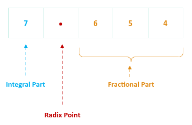
Figure.1
The floating point number consists of the following parts:
Note that the computers deal with numbers in a Base 2 (or binary) format.
The same floating point number above can be approximately represented (up to 3 digits to the right of the radix point) in Base 2 as follows:
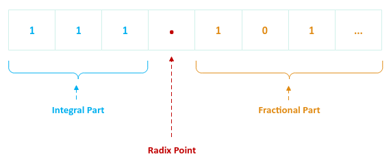
Figure.2
Given that a binary floating point has 3 parts, how is it actually stored in computer's memory ?
This is where the IEEE-754 standards come into play.
The first step is to normalize the binary floating point number to a scientific notation. This
means re-writing the given binary floating point number, such that there is a single non-zero digit to the left of the radix
point, followed by the fractional part and the whole thing multiplied by an exponent part (a power of the base).
For example, the binary floating point number $\color{red}{111.101}$ can be re-written as $\color{red}{1.11101 \times 2^2}$.
Let us look at another example. What about the binary floating point number $\color{red}{0.00101}$ ???
The the binary floating point number $\color{red}{0.00101}$ can be re-written as $\color{red}{1.10100 \times 2^{-3}}$.
The above two examples have been re-written in the normalized binary scientific notation.
From the two examples of the normalized binary floating point number $\color{red}{1.11101 \times 2^2}$ and $\color{red}{1.10100
\times 2^{-3}}$, we can infer that the exponent over the base (2 for binary) can be positive or negative. To simplify the logic of comparing two numbers and not deal with negative numbers, one could
add a constant value (referred to as the bias) to the power of the base, making it an unsigned
biased power.
With the concept of normalization and bias under our belts, now it becomes easy to layout the IEEE-754 standards for storing
floating point numbers.
The following illustration depicts the layout of a Single Precision (32 bits) floating point number:
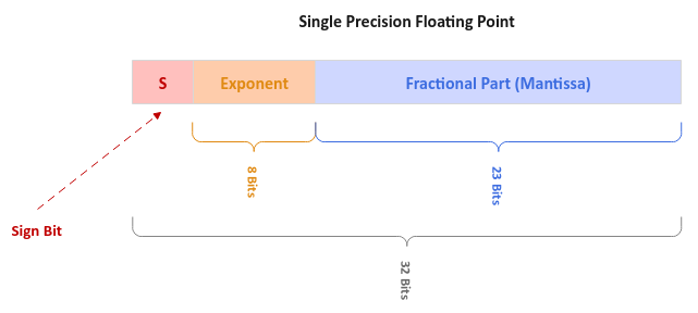
Figure.3
The first bit to the left is the Sign bit with a 0 for positive and a
1 for positive. The next 8 bits are used for the
Exponent (power + bias), and the final set of 23 bits are used for the fractional digits to
the right of the radix point (also referred to as the Mantissa). The bias
value is 127.
The following illustration depicts the layout of a Double Precision (64 bits) floating point number:
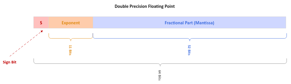
Figure.4
Just the number of bits for the exponent and mantissa are wider. Also, the bias value is 1023.
For the illustration purposes, we will only use single precision floating point representation.
Let us represent the normalized binary floating point number $\color{red}{1.11101 \times 2^2}$ using single precision floating
point representation. We know the bias value is 127. The
power value is $\color{red}{2}$. Therefore, the exponent is $\color{red}{127 + 2} = {129}$.
The binary value for $\color{red}{129}$ is $\color{red}{10000001}$. This is the exponent part in 8 bits. The mantissa part in
23 bits would be the binary value $\color{red}{11101000000000000000000}$.
The following illustration depicts the memory layout of the normalized binary floating point number $\color{red}{1.11101 \times
2^2}$:
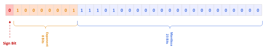
Figure.5
The sign bit is a 0 to represent a positive number.
The following are some facts about the single precision floating point number:
-
If the exponent is all 0s (or $\color{red}{00000000}$) and the
mantissa is all 0s (or $\color{red}{00000000000000000000000}$),
then the single precision floating point value is a 0
-
If the exponent is all 0s (or $\color{red}{11111111}$) and the
mantissa is all 0s (or $\color{red}{00000000000000000000000}$),
then the single precision floating point value is an $\pm\infty$ based on the sign bit
-
If the exponent is all 0s (or $\color{red}{11111111}$) and the
mantissa is NOT 0s, then the single precision floating point value
is an $\textbf{NAN}$
Given a single precision floating point value in the IEEE-754 format, the formula to determine the binary floating point
value is $\color{red}{(-1)^S \times 1.M \times 2^{Exponent-127}}$.
With this we wrap the refresher section on floating point number representation in a computer's memory !!!
As indicated earlier, quantization is the process of reducing the memory size of the model parameters
of a pre-trained LLM model from a higher memory representation format to a lower memory representation
format with minimal loss of information.
The LLM model parameters are typically of type single precision floating point (32 bits). The goal
of quantization is to scale the model parameters to an 8-bit integer.
There are two forms of quantization - the first is linear that maps
the input values to output values using a linear function and the second is
non-linear which maps input values to output values using a non-linear function.
For the quantization of the LLM model parameters, one typically uses a linear quantization techniques,
which involves a Scaling and Rounding operation.
The below are some symbols that will be used in the following section(s):
$\color{red}{r_{min}}$ :: the minimum value of a model parameter (32-bit real number)
$\color{red}{r_{max}}$ :: the maximum value of a model parameter (32-bit real number)
$\color{red}{S}$ :: the scaling factor used to map a model parameter from a 32-bit number system to another $\color
{red}{b}$ bits number system
$\color{red}{Z}$ :: the zero value (0.0) of the model parameter from a 32-bit number system to another $\color{red}
{b}$ bits number system
$\color{red}{X}$ :: the model parameter value (32-bit real value)
$\color{red}{X_q}$ :: the quantized value of a model parameter from a 32-bit value to a b-bit value
The following are the two types of linear quantization techniques:
The absmax quantization technique scales a model parameter from a 32-bit floating point (or
real number) to an 8-bit integer in the range $\color{red}{[-127, 127]}$ and maps the zero value on the 32-bit real number
scale $\color{red}{0.0}$ to the $\color{red}{0}$ on the 8-bit integer scale.
In other words:
$\color{red}{S = \Large{\frac{2^{b-1} - 1}{max(abs(r_{min}, r_{max}))}}}$ $\color{red}{= \Large{\frac{127}{abs(max(r_{min},
r_{max}))}}}$ where $\color{red}{b = 8}$
and
$\color{red}{Z = 0}$
and
$\color{red}{X_q = round(S \times X + Z) = round(S \times X)}$
The following illustration demonstrates this quantization technique for a set of 32-bit numbers to 8-bit numbers:
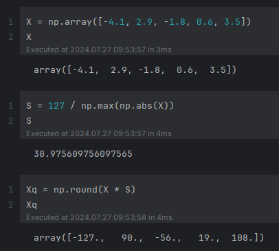
Figure.6
Note that np in the above illustration refers to numpy.
The following illustration depicts the visual for this quantization technique:
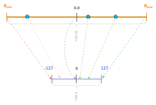
Figure.7
This quantization technique is sometimes is also referred to as Symmetric quantization.
The zeropoint quantization technique scales a model parameter from a 32-bit floating point
(or real number) to an 8-bit integer in the range $\color{red}{[-128, 127]}$ and maps the zero value on the 32-bit floating
point number scale $\color{red}{0.0}$ to a non-zero value on the 8-bit integer scale.
In other words:
$\color{red}{S = \Large{\frac{2^b - 1}{max(r_{min}, r_{max}) - min(r_{min}, r_{max})}}}$ $\color{red}{= \Large{\frac{255}
{{max(r_{min}, r_{max}) - min(r_{min}, r_{max})}}}}$ where $\color{red}{b = 8}$
and
$\color{red}{Z = round(-S \times min(r_{min}, r_{max}) - 2^b)}$
and
$\color{red}{X_q = clip(round(S \times X + Z), -2^b, 2^b-1)}$
The following illustration demonstrates this quantization technique for a set of 32-bit numbers to 8-bit numbers:
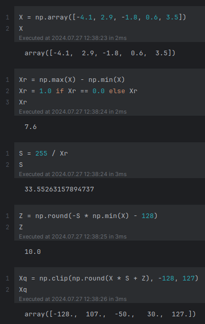
Figure.8
Note that np in the above illustration refers to numpy.
The following illustration depicts the visual for this quantization technique:
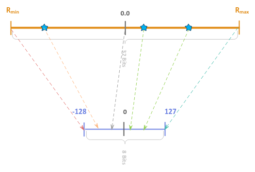
Figure.9
This quantization technique is sometimes is also referred to as Asymmetric quantization.
The setup will be on a Ubuntu 22.04 LTS based Linux desktop. Ensure that the
Python 3.x programming language as well as the Jupyter Notebook packages are installed.
To install the necessary Python packages for this section, execute the following command:
$ pip install bitsandbytes torch transformers
To initialize an instance of the tokenizer, execute the following code snippet:
from transformers import AutoTokenizer

model_name = 'microsoft/Phi-3-mini-4k-instruct'

llm_tokenizer = AutoTokenizer.from_pretrained(model_name)
To initialize an instance of the LLM model, execute the following code snippet:
from transformers import AutoModelForCausalLM

model_name = 'microsoft/Phi-3-mini-4k-instruct'

llm_model = AutoModelForCausalLM.from_pretrained(model_name, torch_dtype='auto', trust_remote_code=True)
To determine the amount of memory comsumed by the LLM model, execute the following code snippet:
print(f'Memory Usage: {round(llm_model.get_memory_footprint()/1024/1024/1024, 2)} GB')
The following typical output:
Output.1
Memory Usage: 7.12 GB
To test the LLM model for text generation, execute the following code snippet:
from transformers import pipeline

prompts = [
  {'role': 'user', 'content': 'Describe what model quantization is all about in a sentence'}
]

pipe = pipeline('text-generation', model=llm_model, tokenizer=llm_tokenizer)

generation_args = {
  'max_new_tokens': 150,
  'return_full_text': False,
  'temperature': 0.0,
  'do_sample': False
}

llm_output = pipe(prompts, **generation_args)
llm_output
The following typical output:
Output.2
[{'generated_text': " Model quantization is the process of reducing the precision of a machine learning model's parameters to decrease its size and computational requirements, while maintaining its performance."}]
This LLM model took about 1 min, 18 secs to execute.
To save the tokenizer as well as the LLM model to a local directory, execute the following code snippet:
model_dir = '/tmp/model'

llm_tokenizer.save_pretrained(model_dir)
llm_model.save_pretrained(model_dir)
To load a quantized instance of the LLM model using 8 bits for the model parameters, execute the following code snippet:
from transformers import BitsAndBytesConfig, AutoModelForCausalLM

model_dir = '/tmp/model'

quantization_config = BitsAndBytesConfig(load_in_8bit=True)

llm_8bit_model = AutoModelForCausalLM.from_pretrained(pretrained_model_name_or_path=model_dir, torch_dtype='auto', quantization_config=quantization_config, trust_remote_code=True)
To determine the amount of memory comsumed by the quantized LLM model, execute the following code snippet:
print(f'Memory Usage: {round(llm_8bit_model.get_memory_footprint()/1024/1024/1024, 2)} GB')
The following typical output:
Output.3
Memory Usage: 3.74 GB
Notice the significant reduction in the memory usage !!!
To test the quantized LLM model for text generation, execute the following code snippet:
from transformers import pipeline

prompts = [
  {'role': 'user', 'content': 'Describe what model quantization is all about in a sentence'}
]

pipe2 = pipeline('text-generation', model=llm_8bit_model, tokenizer=llm_tokenizer)

generation_args = {
    'max_new_tokens': 150,
    'return_full_text': False,
    'temperature': 0.0,
    'do_sample': False
}

llm_output2 = pipe2(prompts, **generation_args)
llm_output2
The following typical output:
Output.4
[{'generated_text': " Model quantization is the process of reducing the precision of a machine learning model's parameters to decrease its memory footprint and computational requirements, often at the cost of some accuracy."}]
This quantized LLM model took about 3 secs to execute and the response was close enough !!!