Univariate Gaussian Distribution Derivation

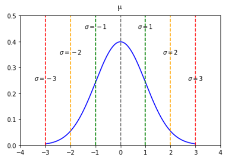
From Statistics, we know that the Gaussian or Normal distribution is a continuous probability distribution with a symmetrical bell-shaped curve plot, such that new samples tend to cluster around the mean ($\mu$) that are within one, two, or three standard deviations ($\sigma$) from the mean ($\mu$).

The following illustration depicts the Gaussian or Normal distribution:

Figure.1

For example, given a typical family, assume the mean height of a female is about $65$ inches and that of a male is about $70$ inches. Given a standard deviation of $2$ inches, a newborn in that family, could grow to a height anywhere between $59$ inches to $76$ inches.

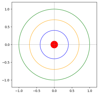
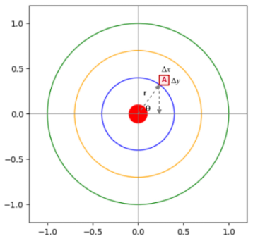
In order to derive the Gaussian or Normal PDF, let us consider a two-dimensional square dart board on the (x, y) coordinate system with the origin (0, 0) at the center (the bullseye) as shown in the illustration below:

Figure.2

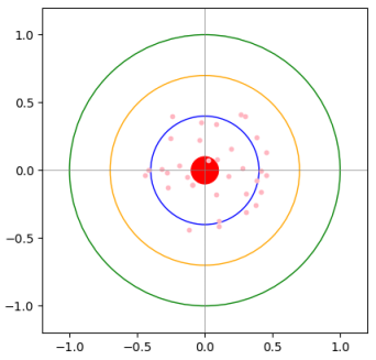
When one throws a dart many number of times, the majority of them will typically land around the center and probably inside the blue circle (in accordance with the Normal distribution) as shown in the illustration below:

Figure.3

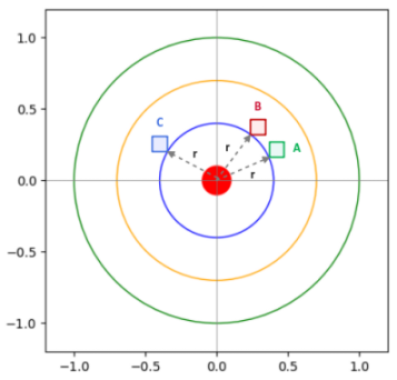
Consider the three regions $A$, $B$, and $C$ along the circumference of the blue circle as shown in the illustration below:

Figure.4

For a dart to land on any point along the circumference of a given circle, the probability will be the same irrespective of the orientation. In other words, from the illustration in Figure.4 above, the probability is the same whether the dart falls in the region $A$, $B$, or $C$.

This also implies that the probability of the dart landing on any coordinate point $(x, y)$ along the circumference of a given circle is NOT influenced by either the $x$ axis or the $y$ axis. They are completely independent of each other.

Assume the throwing of the dart to land in the infinitesimally small red square region $A$ of length $\Delta{x}$ and width $\Delta{y}$ with area $dA = \Delta{x}.\Delta{y}$.

If $r$ is the distance from the origin to the red square region $A$ and if $p(r)$ is the PDF, then the probability of the dart landing in the red square region $A$ is given as follows:

$p(r).dA$ ..... $\color{red}(1)$

Earlier on, we indicated that the position of $x$ is independent of $y$. If we consider a different PDF $f$ in the $(x, y)$ coordinate system, then the probability of the dart landing in the red square region $A$ is given as follows:

$f(x).f(y).dA$ ..... $\color{red}(2)$

The equations $\color{red}(1)$ and $\color{red}(2)$ both are the probability of a dart landing in the red square region $A$.

Therefore, we can arrive at the following equation:

$p(r).dA = f(x).f(y).dA$

Simplifying the above equation, we get:

$p(r) = f(x).f(y)$ ..... $\color{red}(3)$

Now, considering that the dart lands in the red square region $A$, which is $r$ units away from the origin and at an angle $\theta$ from the $x$ axis as shown in the illustration below:

Figure.5

Differentiating the equation (3) with respect to $\theta$ gives us the following equation:

$\Large{\frac{dp(r)}{d\theta}}$ $= \Large{\frac{df(x)}{d\theta}}$ $.f(y) + \Large{\frac{df(y)}{d \theta}}$ $.f(x)$ ..... $\color{red}(4)$

The equation $\color{red}(4)$ can be re-written as follows:

$\Large{\frac{dp(r)}{d\theta}}$ $= \Large{\frac{df(x)}{dx}}$ $.\Large{\frac{dx}{d\theta}}$ $.f(y) + \Large{\frac{df(y)}{dy}}$ $.\Large{\frac{dy}{d\theta}}$ $.f(x)$ ..... $\color{red}(5)$

Since the PDF $p(r)$ is independent of where the dart lands on any point along the circumference of a given circle, it is independent of the angle of rotation $\theta$.

Therefore, we get the following:

$\Large{\frac{dp(r)}{d\theta}}$ $= 0$ ..... $\color{red}(6)$

From the equations $\color{red}(5)$ and $\color{red}(6)$, we get the following:

$\Large{\frac{df(x)}{dx}}$ $.\Large{\frac{dx}{d\theta}}$ $.f(y) + \Large{\frac{df(y)}{dy}}$ $. \Large{\frac{dy}{d\theta}}$ $.f(x)$ $= 0$ ..... $\color{red}(7)$

From Trigonometry, using the information from Figure.5 we get $x = r.cos(\theta)$.

By differentiating the above equation, we get the following:

$\Large{\frac{dx}{d\theta}}$ $= -r.sin(\theta)$ ..... $\color{red}(8)$

Simarly, using the information from Figure.5 we get $y = r.sin(\theta)$.

By differentiating the above equation, we get the following:

$\Large{\frac{dy}{d\theta}}$ $= r.cos(\theta)$ ..... $\color{red}(9)$

The derivative of the PDF $f(x)$ is represented as $\Large{\frac{df(x)}{dx}}$, which can also be represented as $f'(x)$.

Therefore equation $\color{red}(11)$ can be re-written as follows:

$f'(x).(-y).f(y) + f'(y).(x).f(x)$ $= 0$

Simplifying, we get the following:

$x.f(x).f'(y) - y.f'(x).f(y) = 0$

Re-arranging, we get the following:

$x.f(x).f'(y) = y.f'(x).f(y)$ ..... $\color{red}(12)$

Re-arranging the terms in equation $\color{red}(12)$, we get the following:

$\Large{\frac{f'(x)}{x.f(x)}}$ $= \Large{\frac{f'(y)}{y.f(y)}}$ ..... $\color{red}(13)$

We know that the Gaussion or Normal PDF is an exponential distribution function given that it has a bell-shaped curve. From Calculus, we know that the ratio of a function $f(x)$ to its derivative $f'(x)$ for an exponential function is a constant.

For example, consider the following exponential function:

$f(x) = a^x$

Differentiating the above function $f(x)$, we get the following:

$f'(x) = log_e{a}.a^x$

Re-writing the above equation, we get the following:

$f'(x) = log_e{a}.f(x)$

In other words:

$\Large{\frac{f'(x)}{f(x)}}$ $= log_e{a}$

Note that $log_e{a}$ is a constant.

If we use $k$ to represent a constant, then equation $\color{red}(13)$ can be written as follows:

$\Large{\frac{f'(x)}{x.f(x)}}$ $= \Large{\frac{f'(y)}{y.f(y)}}$ $= k$ ..... $\color{red}(14)$

As indicated earlier, both $x$ and $y$ are independent and from equation $\color{red}(14)$, we observe that both $x$ and $y$ differential equations yield the same result of the constant $k$.

So, let us go with $x$ as shown below:

$\Large{\frac{f'(x)}{x.f(x)}}$ $= k$

Re-arranging the aboive equation, we get the following:

$\Large{\frac{f'(x)}{f(x)}}$ $= k.x$ ..... $\color{red}(15)$

Integrating equation $\color{red}(15)$ on both sides, we get the following:

$log_e{f(x)} = \Large{\frac{k.x^2}{2}}$ $+ c$

where $c$ is another constant from the integration.

Applying logarithm on both sides of the above equation, we get the following:

$f(x) = e^{\Large{\frac{k}{2}}.\normalsize{x^2+c}}$

The above equation can be re-written as follows:

$f(x) = e^{\Large{\frac{k}{2}}.\normalsize{x^2}}.e^c$

Given that $e^c$ is some constant, say, $A$, then we get the following:

$f(x) = A.e^{\Large{\frac{k}{2}}.\normalsize{x^2}}$ ..... $\color{red}(16)$

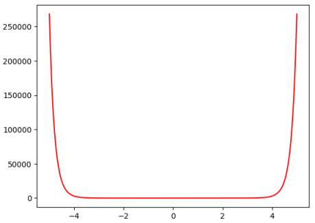
As we can infer from equation $\color{red}(16)$ above, $f(x)$ is an exponential distribution function and its plot is as shown in the illustration below (with $A = 1$ and $k = 1$):

Figure.6

However, the Gaussian or Normal distribution plot is flipped (a beel-curve).

To fix that, we need to introduce a negative sign ($-$) in the exponent of equation $\color{red}(16)$ above, so we get the following:

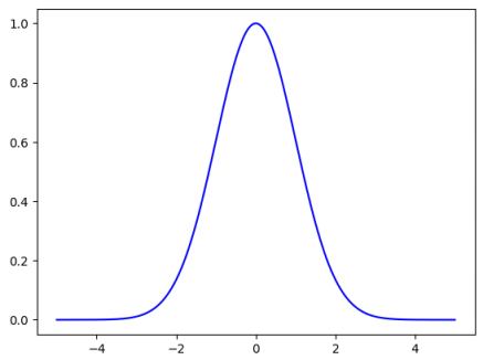
$f(x) = A.e^{-\Large{\frac{k}{2}}.\normalsize{x^2}}$ ..... $\color{red}(17)$

The following illustration depicts the plot of the equation $\color{red}(17)$ (with $A = 1$ and $k = 1$):

Figure.7

YIPPE - we have now figured the foundational exponential function that represents the Gaussian (or Normal) PDF. We still need to determine the values for the constants $A$ and $k$.

Given that we know the total area under a curve for a PDF has to be equal to $1$, we can rewrite equation $\color{red}(17)$ as follows:

$\Large{\int_{\small{-\infty}}^{\small{\infty}}}$ $A.e^{-\Large{\frac{k}{2}}.\normalsize{x^2}} dx = 1$

The above equation can be re-written as follows:

$\Large{\int_{\small{-\infty}}^{\small{\infty}}}$ $e^{-\Large{\frac{k}{2}}.\normalsize{x^2}} dx = \Large{\frac{1}{A}}$

Given that the Gaussian or Normal PDF is symmetrical bell-shaped curve, we can rewrite the above equation as follows:

$2.\Large{\int_{\small{0}}^{\small{\infty}}}$ $e^{-\Large{\frac{k}{2}}.\normalsize{x^2}} dx = \Large{\frac{1}{A}}$

Re-arranging the above equation, we get the following:

$\Large{\int_{\small{0}}^{\small{\infty}}}$ $e^{-\Large{\frac{k}{2}}.\normalsize{x^2}} dx = \Large{\frac{1}{2.A}}$ ..... $\color{red}(18)$

The above equation is not easy to integrate, so we will play a little bit of a trick here.

Squaring on both sides of the above equation, we get the following:

$\Large{(\int_{\small{0}}^{\small{\infty}}}$ $e^{-\Large{\frac{k}{2}}.\normalsize{x^2}} dx \Large {)} \Large{(\int_{\small{0}}^{\small{\infty}}}$ $e^{-\Large{\frac{k}{2}}.\normalsize{x^2}} dx \Large{)} = \Large{\frac{1} {4.A^2}}$

As indicated earlier, both $x$ and $y$ are independent and as observed from equation $\color{red}(14)$, both $x$ and $y$ variables yield the similar results.

Hence we can rewrite the above equation as follows:

Rewriting the above equation, we get the following:

$\Large{\int_{\small{0}}^{\small{\infty}}}$ $\Large{\int_{\small{0}}^{\small{\infty}}}$ $e^{- \Large{\frac{k}{2}}.\normalsize{x^2}}$.$e^{-\Large{\frac{k}{2}}.\normalsize{y^2}} \normalsize{dy\:dx} = \Large{\frac{1} {4.A^2}}$

Simplifying the above equation, we get the following:

$\Large{\int_{\small{0}}^{\small{\infty}}}$ $\Large{\int_{\small{0}}^{\small{\infty}}}$ $e^{- \Large{\frac{k}{2}}.\normalsize{(x^2+y^2)}} \normalsize{dy\:dx} = \Large{\frac{1}{4.A^2}}$ ..... $\color{red}(19)$

Integrating equation $\color{red}(19)$, which is in the $(x, y)$ coordinate system will be very complicated and we could make that easier by moving to the polar coordinate system.

When one transitions from a $(x, y)$ coordinate system to a polar coordinate system, the red square region $A$ becomes more like a segment with an arc, where the length is $\Delta r$ and the width is $r.\Delta \theta$ (because of the arc).

Also, in the $(x, y)$ coordinate system, we are integrating both over the range $(0, \infty)$. In the polar coordinate system, we will have the radius $r$ in the range $(0, \infty)$ and the angle $\theta$ in the range $(0, \Large{\frac{\pi} {2}})$.

With that, we can rewrite equation $\color{red}(19)$ into the polar coordinate system to get the following:

$\Large{\int_{\small{0}}^{\normalsize{\frac{\pi}{2}}}}$ $\Large{\int_{\small{0}}^{\small{\infty}}}$ $e^{-\Large{\frac{k}{2}}.\normalsize{r^2}} \normalsize{.r\:dr\:d{\theta}} = \Large{\frac{1}{4.A^2}}$ ..... $\color{red}(20)$

Let us try to simplify equation $\color{red}(20)$ using the following substitution:

$u = -\Large{\frac{k}{2}}.\normalsize{r^2}$

Differentiating the above equation on both sides, we get the following:

$du = -k.r\:dr$

Re-arranging, we get the following:

$r\:dr = - \Large{\frac{1}{k}}\:\normalsize{du}$

Note that the range of $u$ will be $(0, -\infty)$, since the $u = 0$ when $r = 0$ and $u = -\infty$ when $r = \infty$.

Now to simplify equation $\color{red}(20)$ using $u$, we get the following:

$-\Large{\frac{1}{k}}$ $\Large{\int_{\small{0}}^{\normalsize{\frac{\pi}{2}}}}$ $\Large{\int_{\small {0}}^{\small{-\infty}}}$ $e^{u} \normalsize{\:du\:d{\theta}} = \Large{\frac{1}{4.A^2}}$ ..... $\color{red}(21)$

Let us focus on the following integral term:

$\Large{\int_{\small {0}}^{\small{-\infty}}}$ $e^{u} \normalsize{\:du}$

If $g(u) = e^u$, then we know $g'(u) = e^u$ too. Therefore, the above equation can be re-written as follows:

$\Large{\int_{\small {0}}^{\small{-\infty}}}$ $g'(u) \normalsize{\:du} = g(\infty) - g(0) = e^{ \infty} - e^0 = 0 - 1 = -1$ ..... $\color{red}(22)$

Using the results from equation $\color{red}(22)$ into equation $\color{red}(21)$, we get the following:

$-\Large{\frac{1}{k}}$ $\Large{\int_{\small{0}}^{\normalsize{\frac{\pi}{2}}}}$ $(-1)\:d{\theta} = \Large{\frac{1}{4.A^2}}$ ..... $\color{red}(23)$

The equation $\color{red}(23)$ then reduces to the following:

$\Large{\frac{\pi}{2.k}}$ $= \Large{\frac{1}{4.A^2}}$

Simplifying the above equation, we get the value of $A$ as follows:

$A = \Large{\sqrt{\frac{k}{2.\pi}}}$ ..... $\color{red}(24)$

Substituiting equation $\color{red}(24)$ into equation $\color{red}(17)$, we get the following:

$f(x) = \Large{\sqrt{\frac{k}{2.\pi}}}$ $.e^{-\Large{\frac{k}{2}}.\normalsize{x^2}}$ ..... $\color {red}(25)$

WALLA - the only task now remaining is to find the value for $k$ !!!

Given that the Gaussian or Normal PDF is about the continuous random variable $x$, the next items to discuss would be about the mean ($\mu$) and the standard deviation ($\sigma$).

The mean ($\mu$) for a PDF is defined as the cumulation of all the expected values ($x.f(x)$) in a given range $(-\infty, \infty)$. For Gaussian or Normal PDF, it is defined as follows:

$\Large{\int_{\small {-\infty}}^{\small{\infty}}}$ $\:x.f(x)\:dx$ ..... $\color{red}(26)$

Plugging in equation $\color{red}(25)$ into equation $\color{red}(26)$, we get the following:

$\mu = \Large{\sqrt{\frac{k}{2.\pi}}}$ $\Large{\int_{\small {-\infty}}^{\small{\infty}}}$ $x.e^{- \Large{\frac{k}{2}}.\normalsize{x^2}}\:dx$ ..... $\color{red}(27)$

Equation $\color{red}(27)$ is an odd function since we have both the odd term $x$ and the even term $x^2$ and as a result every value of $x$ in the range $(-\infty, 0)$ will cancel out with every value of $x$ in the range $(0, \infty)$ due to the symmetrical nature of the Gaussian or Normal PDF.

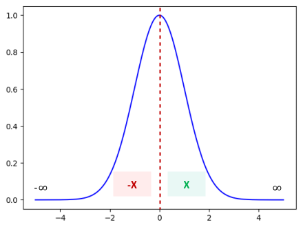
The following illustration depicts this situation:

Figure.8

The cummulative expected value in the region X cancel out the cummulative expected value in the region -X.

Hence, the mean ($\mu$) of the Gaussian or Normal PDF is zero ($0$).

Moving on to the variance ($\sigma^{2}$) for the Gaussian or Normal PDF.

The variance ($\sigma^{2}$) for a PDF is defined as the cumulation of all the expected values [$(x-\mu)^2.f(x)$] in a given range $(-\infty, \infty)$. For Gaussian or Normal PDF, it is defined as follows:

$\Large{\int_{\small {-\infty}}^{\small{\infty}}}$ $\:(x-\mu)^2.f(x)\:dx$

Given that the mean ($\mu$) is equal to $0$, we can rewrite the above equation as follows:

$\Large{\int_{\small {-\infty}}^{\small{\infty}}}$ $\:x^2.f(x)\:dx$ ..... $\color{red}(28)$

Plugging in equation $\color{red}(25)$ into equation $\color{red}(28)$, we get the following:

$\sigma^{2} = \Large{\sqrt{\frac{k}{2.\pi}}}$ $\Large{\int_{\small {-\infty}}^{\small{\infty}}}$ $x^2.e^{-\Large{\frac{k}{2}}.\normalsize{x^2}}\:dx$

We know that the Gaussian or Normal PDF is symmetrical curve, so we can rewrite the above equation as follows:

$\sigma^{2} = 2.\Large{\sqrt{\frac{k}{2.\pi}}}$ $\Large{\int_{\small {0}}^{\small{\infty}}}$ $x^2.e^{-\Large{\frac{k}{2}}.\normalsize{x^2}}\:dx$

We can rewrite the above equation as follows:

$\sigma^{2} = 2.\Large{\sqrt{\frac{k}{2.\pi}}}$ $\Large{\int_{\small {0}}^{\small{\infty}}}$ $x.x.e^{-\Large{\frac{k}{2}}.\normalsize{x^2}}\:dx$ ..... $\color{red}(29)$

To solve the equation $\color{red}(29)$, we will use the technique called Integration by Parts, which uses the following formula:

$\Large{\int}$ $\:u\:dv = u.v\:-$ $\Large{\int}$ $\:v\:du$ ..... $\color{red}(30)$

Let us assign $u$ the following value:

$u = x$..... $\color{red}(31)$

By differentiating both sides of equation $\color{red}(31)$, we get the following:

$du = dx$ ..... $\color{red}(32)$

Similarly, let us assign $dv$ the following value:

$dv = x.e^{-\Large{\frac{k}{2}}.\normalsize{x^2}}$..... $\color{red}(33)$

By integrating both sidesof the equation $\color{red}(33)$, we get the following:

$v = -\Large{\frac{1}{k}}$ $e^{-\Large{\frac{k}{2}}.\normalsize{x^2}}$ ..... $\color{red}(34)$

With $u$ and $dv$ defined as in equations $\color{red}(31)$ and $\color{red}(33)$, the integration part of equation $\color {red}(29)$ is in the form of equation $\color{red}(30)$ and can be re-written as follows:

$\sigma^{2} = 2.{\sqrt{\frac{k}{2.\pi}}}$ $\Large{[}$ $-\Large{\frac{x}{k}}$ $.e^{-\Large{\frac{k} {2}}.\normalsize{x^2}}$ $\Large{\rvert_{\small0}^{\small\infty}}$ $+ \Large{\frac{1}{k}}$ $\Large{\int_{\small {0}}^{\small {\infty}}}$ $e^{-\Large{\frac{k}{2}}.\normalsize{x^2}}\:dx$ $\Large{]}$ ..... $\color{red}(35)$

Note that the symbol $\Large{\rvert_{\small0}^{\small\infty}}$ is referred to as the integral Evaluation Bar at the two limits $0$ and $\infty$.

The first term $-\Large{\frac{x}{k}}$ $.e^{-\Large{\frac{k}{2}}.\normalsize{x^2}}$ $\Large{\rvert_{\small0}^{\small\infty}}$ of the equation $\color{red}(35)$ basically evaluates to a zero ($0$) because for $x = 0$, the term is $0$ and for $x = \infty$, $e^{\infty}$ is $0$. Hence, the first term drops off and the equation simply becomes the following:

$\sigma^{2} = 2.{\sqrt{\frac{k}{2.\pi}}}$ $\Large{[}$ $\Large{\frac{1}{k}}$ $\Large{\int_{\small {0}} ^{\small{\infty}}}$ $e^{-\Large{\frac{k}{2}}.\normalsize{x^2}}\:dx$ $\Large{]}$ ..... $\color{red}(36)$

From equation $\color{red}(18)$, we know the integral term of the equation $\color{red}(36)$ equals $\Large{\frac{1}{2.A}}$.

Therefore, the equation $\color{red}(36)$ can be written as follows:

$\sigma^{2} = 2.{\sqrt{\frac{k}{2.\pi}}}$ $.\Large{\frac{1}{k}}$ $.\Large{\frac{1}{2.A}}$ ..... $\color{red}(37)$

From equation $\color{red}(24)$, we know the value for $A$.

Therefore the equation $\color{red}(37)$ can be written as follows:

$\sigma^{2} = 2.{\sqrt{\frac{k}{2.\pi}}}$ $.\Large{\frac{1}{2.k}}$ $.{\sqrt{\frac{2.\pi}{k}}}$

Simplifying the above equation, we get the following:

$k = \Large{\frac{1}{\sigma^2}}$ ..... $\color{red}(38)$

Substituiting equation $\color{red}(38)$ into equation $\color{red}(25)$, we get the following:

$f(x) = \Large{\frac{1}{\sigma\sqrt{2.\pi}}}$ $e^{-\frac{1}{2}.(\frac{x}{\sigma})^2}$.

Given that the mean ($\mu$) is zero ($0$) in our case for Gaussian or Normal PDF, one can rewrite the above equation as follows:

$f(x) = \Large{\frac{1}{\sigma\sqrt{2.\pi}}}$ $e^{-\frac{1}{2}.(\frac{x-\mu}{\sigma})^2}$.

BINGO !!! We have successfully derived the equation for the Gaussian or Normal PDF !!!